Multiple Linear Regression Analysis of Temperature Data in Albany and Sacramento
Introduction
The study of weather patterns has been of great interest to scientists, researchers and the general public for many years. In recent times, there has been a growing concern about the impacts of global warming and climate change on weather patterns and the environment. One area of particular interest is the relationship between temperature and other meteorological variables, such as humidity, precipitation, and wind speed. Understanding this relationship is important for improving our understanding of climate patterns and predicting future weather patterns. This study aims to investigate the relationship between temperature and the other meteorological variables in the United States, and to explore how this relationship varies across a specific time range.
The dataset pertains to two prominent cities located on the opposite coasts of the United States: Albany, the capital city of New York State, and Sacramento, the capital city of California State. The data were respectively collected from Albany International Airport and Sacramento Metropolitan Airport.
The data was extracted from the National Oceanic and Atmospheric Administration (NOAA) website on 5 May 2023 and is a subset of the Local Climatological Data (LCD) dataset. The original data ranges back to the 1940s and 1970s for the two selected stations, but for the purpose of this report, we will be analyzing measurements from January 1st, 2000, to December 31st, 2022.
The data was stored in two seperate csv files. It is worth noting that the Daily Humidity values in Sacramento are only available from January 1st, 2005. The data was parsed, cleaned and slightly pre-processed in Excel.
It is worth noting the units of measurement employed for the various variables under consideration. Temperature is expressed in Celsius, wind speed in meters per second (m/s), precipitation in millimeters (mm), and humidity in percentage (%).
The study was conducted utilizing Python 3 and Jupyter Notebook as the programming and development environment. To ensure clarity, comprehensibility, and reproducibility, the report incorporates the code implementation and its corresponding outputs. This approach facilitates a transparent presentation of the analysis, enabling us to follow the methodology and reproduce the results beyond the final report .
Exploratory data analysis: Understanding the data
# Importing libraries
import matplotlib.pyplot as plt
import pandas as pd
import numpy as np
import seaborn as sns
from matplotlib.dates import MonthLocator, DateFormatter
import statsmodels.api as sm
# Reading the datasets
albany = pd.read_csv('albany.csv')
sacramento = pd.read_csv('sacramento.csv')
# Datetime formatting
sacramento['date'] = pd.to_datetime(sacramento['date'], format='%d/%m/%Y')
albany['date'] = pd.to_datetime(albany['date'], format='%d/%m/%Y')
The tail() method in the code below is used to retrieve the last rows of the Sacramento DataFrame. This feature facilitates rapid examination of the end of DataFrame, enabling data verification. We confirm the presence of 8333 rows and 7 columns, which include the date variable.
print (sacramento.tail(), "\n The size of the DataFrame is", sacramento.shape)
           date  averagetemperature  averagewindspeed  maximumtemperature  \
8329 2022-12-27               10.56              6.84               12.78
8330 2022-12-28                6.11              1.48               10.00
8331 2022-12-29               10.00              3.98               12.22
8332 2022-12-30               13.89              8.18               16.67
8333 2022-12-31               13.33              7.82               15.56

      minimumtemperature  precipitation  humidity
8329                8.33          10.41     85.33
8330                2.22           0.00     90.75
8331                7.22          16.26     85.04
8332               11.11           1.52     87.71
8333               10.56          47.75     82.71
 The size of the DataFrame is (8334, 7)
We proceed to do the same with the Albany DataFrame, and confirm the presence of 8375 rows and 7 columns.
print (albany.tail(), "\n The size of the DataFrame is", albany.shape)
           date  averagetemperature  averagewindspeed  maximumtemperature  \
8370 2022-12-27               -2.22              2.59                1.11
8371 2022-12-28                0.00              3.04                5.00
8372 2022-12-29                1.67              2.59                8.89
8373 2022-12-30               10.00              3.53               13.89
8374 2022-12-31                9.44              3.80               11.67

      minimumtemperature  precipitation  humidity
8370               -5.56           0.00     56.88
8371               -5.56           0.00     63.63
8372               -5.56           0.00     61.33
8373                6.11           0.00     52.79
8374                6.67           2.03     81.17
 The size of the DataFrame is (8375, 7)
In the following, the describe() method, particularly useful for exploratory data analysis, allows for a comprehensive understanding of the data’s summary statistics at a glance. These statistics provide insights into the central tendency, variability, and distribution of the data in each column of the DataFrame.
Sacramento
sacramento.describe()
| averagetemperature | averagewindspeed | maximumtemperature | minimumtemperature | precipitation | humidity | |
|---|---|---|---|---|---|---|
| count | 8334.000000 | 8334.000000 | 8334.000000 | 8334.000000 | 8334.000000 | 6572.000000 |
| mean | 16.758523 | 3.378572 | 24.091746 | 9.145821 | 1.173276 | 63.278203 |
| std | 6.681999 | 1.715114 | 8.657389 | 5.392560 | 4.735319 | 16.252343 |
| min | 0.560000 | 0.040000 | 3.890000 | -11.110000 | 0.000000 | 16.000000 |
| 25% | 11.110000 | 2.100000 | 16.670000 | 5.000000 | 0.000000 | 51.040000 |
| 50% | 16.670000 | 3.170000 | 23.890000 | 9.440000 | 0.000000 | 62.130000 |
| 75% | 22.780000 | 4.430000 | 31.670000 | 13.330000 | 0.000000 | 76.250000 |
| max | 35.560000 | 13.500000 | 53.890000 | 27.220000 | 104.650000 | 100.000000 |
In Sacramento, California, the average annual temperature is around 16.76 degrees Celsius, with a standard deviation of approximately 6.68. The temperature range is substantial, indicating potential fluctuations in weather conditions. Notably, the highest recorded temperature of 53.89 degrees Celsius occurred on March 19, 2018, while the lowest temperature of -11.11 degrees Celsius was recorded on February 11, 2004.
Likewise, the average precipitation amount in Sacramento is approximately 1.17 mm. The precipitation values demonstrate a standard deviation of about 4.74 units. This aligns with the prevailing climate in California, characterized by hot, arid summers and short, cold, wet winters, resulting in partly cloudy conditions. The number of days with precipitations below the average overall precipitation amount of 1.17 mm is 7368 days, over the study period of 8334 days.
The descriptive measures of central tendency and variability correspond to the anticipated weather patterns in the area.
max_temp_index = sacramento['maximumtemperature'].idxmax()
date_max_temp = sacramento.loc[max_temp_index, 'date']
min_temp_index = sacramento['minimumtemperature'].idxmin()
date_min_temp = sacramento.loc[min_temp_index, 'date']
print("Date with the highest maximum temperature:", date_max_temp)
print("Date with the lowest minimum temperature:", date_min_temp)
Date with the highest maximum temperature: 2018-03-19 00:00:00
Date with the lowest minimum temperature: 2004-02-11 00:00:00
count_below_threshold = sacramento[sacramento['precipitation'] < 1.17].shape[0]
print("Number of days with precipitations below the average precipitation amount of 1.17 mm is :", count_below_threshold)
count_exceeding_threshold = sacramento[sacramento['averagetemperature'] > 16.76].shape[0]
print("Number of days with daily average temperature exceeding the overall average temperature of 9.92 C is :", count_exceeding_threshold)
Number of days with precipitations below the average precipitation amount of 1.17 mm is : 7368
Number of days with daily average temperature exceeding the overall average temperature of 9.92 C is : 4028
columns_to_include = ['averagetemperature', 'averagewindspeed', 'precipitation', 'humidity']
subset_sacramento = sacramento[columns_to_include]
# pair plots between numerical columns
sns.pairplot(subset_sacramento)
plt.show()
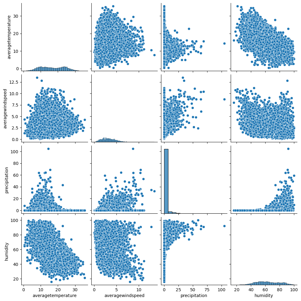
The grid figure presented illustrates the pair plots, providing insights into the relationships, distributions, and interactions among the selected variables. These visualizations allow for a better understanding of the anticipated effects of each variable on the target temperature variable. To enhance the visual clarity of the plots, the minimum and maximum temperatures were excluded from the analysis.
An evident observation is the strong negative correlation between humidity and average temperature, with a limited number of noticeable outliers. In contrast, the relationship between precipitation and temperature does not exhibit a clear pattern, but rather displays more outlier values. Notably, low precipitation values are observed across various temperature ranges, whereas higher precipitation values tend to occur within a specific temperature range.
Furthermore, the influence of wind speed on temperature is not evident for lower wind speed values. However, as the wind speed increases, the temperature tends to stabilize within a specific temperature range. This finding suggests that wind speed may serve as a more reliable predictor of temperature within this specific range.
Overall, the pair plots provide valuable insights into the relationships and patterns among the variables, shedding light on their potential impact on the studied temperature variable.
correlation_matrix = sacramento.corr()
sns.heatmap(correlation_matrix, annot=True, cmap="coolwarm")
plt.title("Sacramento Correlation Matrix Heatmap")
plt.show()
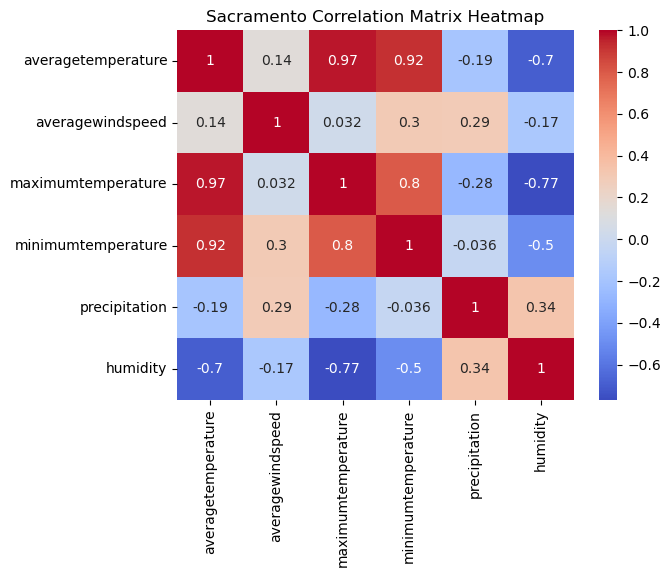
The heatmap figure provides a visual representation of the correlation coefficients between pairs of variables. Each cell in the heatmap represents the correlation coefficient, with color gradients indicating the magnitude and direction of the correlation. Warmer colors, such as shades of red, indicate a positive correlation, while cooler colors, such as shades of blue, indicate a negative correlation.
The heatmap reinforces the observations made from the pair plots mentioned earlier. It visually confirms the relationships and patterns observed between variables.
Furthermore, in the process of building our model, we have made the decision to only include the minimum temperature variable and exclude the maximum temperature. This decision is based on the redundancy of their influence on the average temperature and the potential issue of multicollinearity that could arise. By excluding the maximum temperature, we aim to prevent any redundant or collinear effects in our analysis.
Albany
albany.describe()
| averagetemperature | averagewindspeed | maximumtemperature | minimumtemperature | precipitation | humidity | |
|---|---|---|---|---|---|---|
| count | 8330.000000 | 8330.000000 | 8330.000000 | 8330.000000 | 8331.000000 | 8375.000000 |
| mean | 9.916845 | 3.286505 | 15.062441 | 4.494155 | 2.862368 | 68.329931 |
| std | 10.551006 | 1.709147 | 11.239033 | 10.239078 | 7.307641 | 12.755930 |
| min | -21.670000 | 0.000000 | -17.780000 | -26.670000 | 0.000000 | 24.710000 |
| 25% | 1.670000 | 2.010000 | 5.560000 | -2.780000 | 0.000000 | 59.960000 |
| 50% | 10.560000 | 3.080000 | 16.110000 | 4.440000 | 0.000000 | 68.250000 |
| 75% | 19.440000 | 4.290000 | 25.000000 | 13.330000 | 1.780000 | 77.500000 |
| max | 31.110000 | 10.590000 | 37.220000 | 25.000000 | 119.130000 | 100.000000 |
In Albany, New York, the average overall temperature is around 9.92 degrees Celsius, with a standard deviation of approximately 10.55. The temperature range is as substantial as in Sacramento (around 64 degrees Celsius between the lowest and highest values in both), indicating potential fluctuations in weather conditions. Notably, the highest recorded temperature of 37.22 degrees Celsius occurred on July 21, 2011, while the lowest temperature of -26.67 degrees Celsius was recorded on January 24, 2005.
Likewise, the average precipitation amount in Albany is approximately 2.86 mm. The precipitation values demonstrate a standard deviation of about 7.3 units.
This aligns with the prevailing climate in New York, characterized by humid continental with warm to hot summers and freezing cold snowy winters. The number of days with precipitations below the average overall precipitation amount of 2.86 mm is 6603 days, over the study data of 8330 days. While the number of days with daily average temperatures exceeding the overall average temperature of 9.92 C was 4318 days. The descriptive measures of central tendency and variability correspond to the anticipated weather patterns in the area.
These findings from both areas suggest that in comparison, most precipitations in Sacramento occured in fewer days that had an excessive amount of pecipitations. In contrast, the precipitations in Albany were better spread over more days.
max_temp_index2 = albany['maximumtemperature'].idxmax()
date_max_temp2 = albany.loc[max_temp_index2, 'date']
min_temp_index2 = albany['minimumtemperature'].idxmin()
date_min_temp2 = albany.loc[min_temp_index2, 'date']
print("Date with the highest maximum temperature:", date_max_temp2)
print("Date with the lowest minimum temperature:", date_min_temp2)
Date with the highest maximum temperature: 2011-07-21 00:00:00
Date with the lowest minimum temperature: 2005-01-24 00:00:00
count_below_threshold = albany[albany['precipitation'] < 2.86].shape[0]
print("Number of days with precipitations below the average precipitation amount of 2.86 mm is :", count_below_threshold)
count_exceeding_threshold = albany[albany['averagetemperature'] > 9.92].shape[0]
print("Number of days with daily average temperature exceeding the overall average temperature of 9.92 C is :", count_exceeding_threshold)
Number of days with precipitations below the average precipitation amount of 2.86 mm is : 6603
Number of days with daily average temperature exceeding the overall average temperature of 9.92 C is : 4318
subset_albany = albany[columns_to_include]
# pair plots between numerical columns
sns.pairplot(subset_albany)
plt.show()
correlation_matrix2 = albany.corr()
sns.heatmap(correlation_matrix2, annot=True, cmap="coolwarm")
plt.title("Albany Correlation Matrix Heatmap")
plt.show()
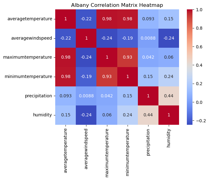
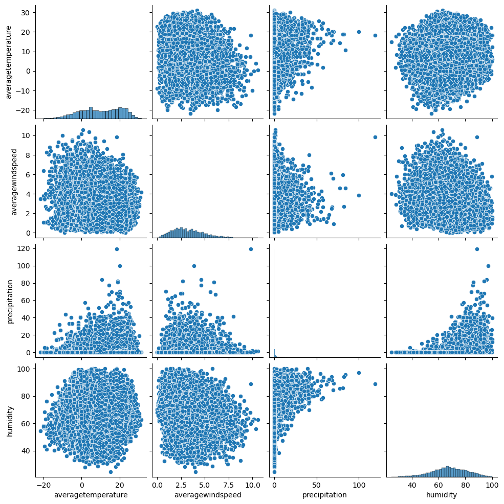
The pair plots and heatmap figures for Albany, New York, reveal distinct patterns and relationships among the variables. A notable observation is the prevalence of low correlation coefficients and cooler colors in the heatmap, indicating weaker associations between the variables.
In particular, the maximum and minimum temperatures exhibit a strong positive correlation with the average temperature, suggesting a consistent relationship between these variables. However, for humidity and windspeed, there are no discernible patterns or clear correlations with the average temperature. Additionally, there are several outliers observed in the precipitation variable, indicating instances of extreme or unusual precipitation values.
The absence of clear patterns and the presence of non-linear relationships between humidity, precipitation, windspeed, and average temperature in Albany, New York, can be attributed to the specific nature of the local climate category. This climate category is described as humid continental, characterized by warm to hot summers and freezing cold snowy winters.
Within this climate category, the intricate interplay among various atmospheric conditions, such as prevailing winds and moisture sources, gives rise to diverse and dynamic weather patterns. The variability in temperature, humidity, precipitation, and windspeed is influenced by numerous factors and regional weather phenomena, including blizzards. Furthermore, the seasonal temperature extremes and the potential impact of the proximity to large bodies of water, such as the Atlantic Ocean, introduce additional variability and non-linear relationships among the variables under study.
Considering the distinct characteristics of the locality, it is reasonable to expect that the relationships may not conform to a simple linear pattern. The complex interplay of factors such as temperature inversions, air masses, and local topography contributes to the observed complexity in these relationships.
Multiple linear regression
Sacramento
sacramento.isnull().sum()
date                     0
averagetemperature       0
averagewindspeed         0
maximumtemperature       0
minimumtemperature       0
precipitation            0
humidity              1762
dtype: int64
Prior to constructing the linear regression model, we examine the dataset for missing values. As a result, we identify 1762 instances of missing data specifically pertaining to the humidity variable. Instead of discarding these unavailable data points, which represent a substantial portion of the entire dataset, we opted to impute the missing values using the mean.
mean_humidity = sacramento['humidity'].mean()
sacramento['humidity'].fillna(mean_humidity, inplace=True)
# Adding a constant column to the independent variables:
# in the context of using statsmodels for multiple linear regression, it represents the intercept term in the linear regression equation
X = sacramento[['averagewindspeed', 'minimumtemperature', 'precipitation', 'humidity']]
X = sm.add_constant(X)

# Defining the dependent variable
y = sacramento['averagetemperature']

# Fitting the OLS model
model = sm.OLS(y, X)
results = model.fit()

# Print the regression summary
print(results.summary())
                            OLS Regression Results
==============================================================================
Dep. Variable:     averagetemperature   R-squared:                       0.926
Model:                            OLS   Adj. R-squared:                  0.926
Method:                 Least Squares   F-statistic:                 2.601e+04
Date:                Sun, 18 Jun 2023   Prob (F-statistic):               0.00
Time:                        23:27:19   Log-Likelihood:                -16811.
No. Observations:                8334   AIC:                         3.363e+04
Df Residuals:                    8329   BIC:                         3.367e+04
Df Model:                           4
Covariance Type:            nonrobust
======================================================================================
                         coef    std err          t      P>|t|      [0.025      0.975]
--------------------------------------------------------------------------------------
const                 16.2143      0.133    121.559      0.000      15.953      16.476
averagewindspeed      -0.5312      0.013    -40.981      0.000      -0.557      -0.506
minimumtemperature     1.0532      0.004    245.554      0.000       1.045       1.062
precipitation         -0.0711      0.005    -15.089      0.000      -0.080      -0.062
humidity              -0.1139      0.002    -69.456      0.000      -0.117      -0.111
==============================================================================
Omnibus:                      663.002   Durbin-Watson:                   0.920
Prob(Omnibus):                  0.000   Jarque-Bera (JB):             3431.099
Skew:                          -0.189   Prob(JB):                         0.00
Kurtosis:                       6.121   Cond. No.                         439.
==============================================================================

Notes:
[1] Standard Errors assume that the covariance matrix of the errors is correctly specified.
The OLS Regression Results provide insights into the linear regression model that was applied to the dataset. The R-squared value of 0.926 indicates that approximately 92.6% of the variability in the average temperature (dependent variable) can be accounted for by the independent variables included in the model. This suggests a robust relationship between the independent variables (averagewindspeed, minimumtemperature, precipitation, humidity) and the average temperature.
The F-statistic is 2.601e+04, with a remarkably low probability (p < 0.001). This implies that the overall regression model is statistically significant, indicating that at least one of the independent variables exhibits a significant association with the average temperature.
The coefficients represent the estimated impact of each independent variable on the average temperature while holding other variables constant. Here are the interpretations of the coefficients:
- average windspeed: With each unit increase in average windspeed, the average temperature is estimated to decrease by approximately 0.5312 units.
- minimum temperature: With each unit increase in minimum temperature, the average temperature is estimated to increase by approximately 1.0532 units.
- precipitation: With each unit increase in precipitation, the average temperature is estimated to decrease by approximately 0.0711 units.
- humidity: With each unit increase in humidity, the average temperature is estimated to decrease by approximately 0.1139 units.
The p-values associated with each coefficient are very low (p < 0.001), indicating that all independent variables have a statistically significant relationship with the average temperature.
The 95% confidence intervals provide a range within which the true value of each coefficient is likely to fall. For example, the confidence interval for the average windspeed coefficient is (-0.557, -0.506), suggesting that the true effect of average windspeed on average temperature lies within this range with 95% confidence.
Overall, the findings support the idea that the independent variables (averagewindspeed, minimumtemperature, precipitation, humidity) are significant predictors of the average temperature in the Sacramento dataset. The regression model has a high R-squared value, indicating a good fit, and the coefficients and p-values suggest that all independent variables have a meaningful impact on the average temperature.
The regression equation is:
# Obtain the predicted values
y_pred = results.predict(X)

# Calculate the residuals
residuals = y - y_pred

# Plot the Residuals vs. Fitted values
sns.residplot(x=y_pred, y=residuals, lowess=True, line_kws={'color': 'red'})
plt.xlabel('Fitted Values')
plt.ylabel('Residuals')
plt.title('Residuals vs. Fitted Values')
plt.show()
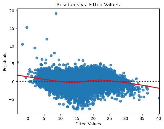
The (Residuals vs. Fitted) plot shows that the residuals are fairly randomly scattered around the 0 residual line. Also, the residuals form a seemingly horizontal band around the residual = 0 line, which suggests that the variances of the error terms can be considered equal.
The graph shows a number of outliers that deviate significantly from the general pattern of the residuals and could be investigated further. The number of these individual points shouldn’t greatly impact the regression coefficients and overall model fit.
# Generate the normal QQ plot
sm.qqplot(residuals, line='s')
plt.title('Normal QQ Plot of Residuals')
plt.show()
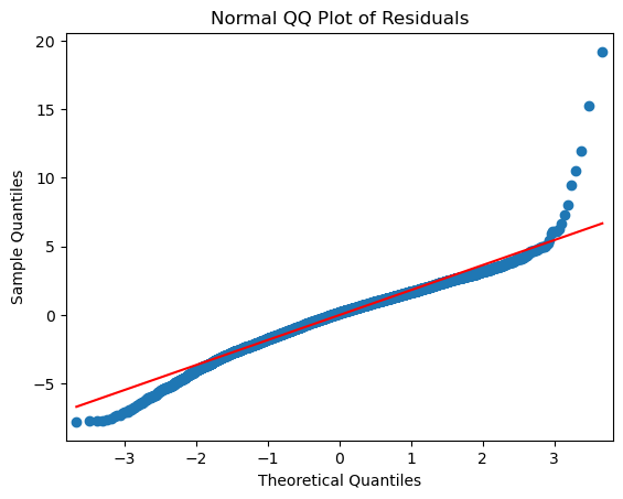
The (Normal Q-Q) plot shows if residuals are normally distributed (with a small tail). The relationship between the theoretical quantiles and the standardized residuals is approximately linear for most points. We can say that the error terms are indeed normally distributed. The presence of some outliers is confirmed and pronounced here as well.
Albany
albany.isnull().sum()
date                   0
averagetemperature    45
averagewindspeed      45
maximumtemperature    45
minimumtemperature    45
precipitation         44
humidity               0
dtype: int64
Similar to Sacramento, we examine the dataset for missing values. We identify at most 45 instances of missing data pertaining to all variables except for humidity. We can proceed to discarding these unavailable data points, which do not represent a substantial portion of the entire dataset.
albany.dropna(inplace=True)
X2 = albany[['averagewindspeed', 'minimumtemperature', 'precipitation', 'humidity']]
X2 = sm.add_constant(X2)

# Defining the dependent variable
y2 = albany['averagetemperature']

# Fitting the OLS model
model2 = sm.OLS(y2, X2)
results2 = model2.fit()

# Print the regression summary
print(results2.summary())
                            OLS Regression Results
==============================================================================
Dep. Variable:     averagetemperature   R-squared:                       0.972
Model:                            OLS   Adj. R-squared:                  0.972
Method:                 Least Squares   F-statistic:                 7.188e+04
Date:                Sun, 18 Jun 2023   Prob (F-statistic):               0.00
Time:                        23:27:28   Log-Likelihood:                -16575.
No. Observations:                8330   AIC:                         3.316e+04
Df Residuals:                    8325   BIC:                         3.320e+04
Df Model:                           4
Covariance Type:            nonrobust
======================================================================================
                         coef    std err          t      P>|t|      [0.025      0.975]
--------------------------------------------------------------------------------------
const                 12.0641      0.134     89.777      0.000      11.801      12.328
averagewindspeed      -0.3560      0.012    -29.811      0.000      -0.379      -0.333
minimumtemperature     1.0241      0.002    519.140      0.000       1.020       1.028
precipitation         -0.0116      0.003     -3.895      0.000      -0.018      -0.006
humidity              -0.0812      0.002    -45.519      0.000      -0.085      -0.078
==============================================================================
Omnibus:                      805.064   Durbin-Watson:                   1.529
Prob(Omnibus):                  0.000   Jarque-Bera (JB):             1700.446
Skew:                           0.618   Prob(JB):                         0.00
Kurtosis:                       4.836   Cond. No.                         484.
==============================================================================

Notes:
[1] Standard Errors assume that the covariance matrix of the errors is correctly specified.
The R-squared value of 0.972 indicates that approximately 97.2% of the variability in the average temperature (dependent variable) can be accounted for by the independent variables included in the model. This suggests a strong relationship between the independent variables (averagewindspeed, minimumtemperature, precipitation, humidity) and the average temperature.
The F-statistic is 7.188e+04, with a remarkably low probability (p < 0.001). This implies that the overall regression model is highly statistically significant, indicating that at least one of the independent variables exhibits a significant association with the average temperature.
The coefficients represent the estimated impact of each independent variable on the average temperature while holding other variables constant. Here are the interpretations of the coefficients:
- average windspeed: With each unit increase in average windspeed, the average temperature is estimated to decrease by approximately 0.3560 units.
- minimum temperature: With each unit increase in minimum temperature, the average temperature is estimated to increase by approximately 1.0241 units.
- precipitation: With each unit increase in precipitation, the average temperature is estimated to decrease by approximately 0.0116 units.
- humidity: With each unit increase in humidity, the average temperature is estimated to decrease by approximately 0.0812 units.
The p-values associated with each coefficient are very low (p < 0.001), indicating that all independent variables have a statistically significant relationship with the average temperature.
The 95% confidence intervals provide a range within which the true value of each coefficient is likely to fall. For example, the confidence interval for the average windspeed coefficient is (-0.379, -0.333), suggesting that the true effect of average windspeed on average temperature lies within this range with 95% confidence.
The OLS Regression Results show that the regression model has a high R-squared value of 0.972, indicating that approximately 97.2% of the variability in the average temperature (dependent variable) can be explained by the independent variables included in the model. The F-statistic of 7.188e+04 is highly significant (p < 0.001), indicating that the overall regression model is statistically significant.
The regression equation can be expressed as:
# Obtain the predicted values
y_pred2 = results2.predict(X2)

# Calculate the residuals
residuals2 = y2 - y_pred2

# Plot the Residuals vs. Fitted values
sns.residplot(x=y_pred2, y=residuals2, lowess=True, line_kws={'color': 'red'})
plt.xlabel('Fitted Values')
plt.ylabel('Residuals')
plt.title('Residuals vs. Fitted Values')
plt.show()
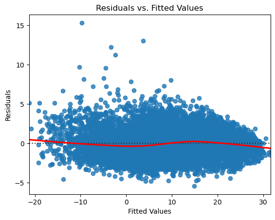
Also in this case, the (Residuals vs. Fitted) plot shows that the residuals are randomly scattered around the 0 residual line. The residuals form a horizontal band around the residual = 0 line, which suggests that the variances of the error terms are considered equal.
The graph shows a number of outliers that deviate significantly from the general pattern of the residuals and could be investigated further. The number of these individual points wouldn’t greatly impact the regression coefficients and overall model fit.
# Generate the normal QQ plot
sm.qqplot(residuals2, line='s')
plt.title('Normal QQ Plot of Residuals')
plt.show()
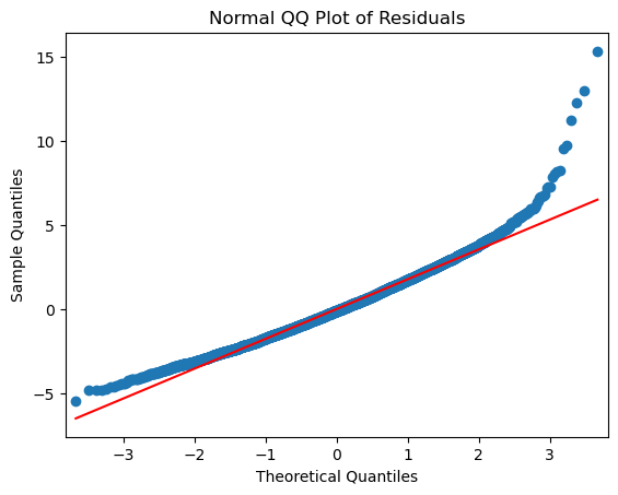
The (Normal Q-Q) plot shows that the relationship between the theoretical quantiles and the standardized residuals is approximately linear for most points. However, it is in fact skewed right, meaning that most of the data is distributed on the left side with a long “tail” of data extending out to the right. The points depart upward from the straight red line as you follow the quantiles from left to right. The red line shows where the points would fall if the dataset were normally distributed. The point’s trend upward shows that the actual quantiles are much greater than the theoretical quantiles, meaning that there is a greater concentration of data beyond the right side of a Gaussian distribution.
Overall, the findings derived from the linear regression analysis provide evidence supporting the existence of a relationship between temperature and meteorological variables in the United States, with a specific focus on Albany and Sacramento. Both cities exhibit statistically significant associations between temperature and the meteorological variables of average windspeed, minimum temperature, precipitation, and humidity.
By understanding and analyzing these relationships, we can enhance our understanding of weather patterns, contribute to climate studies, and improve weather predictions. These findings highlight the significance of considering multiple meteorological factors when examining temperature variations and provide valuable insights into the impacts of these variables on weather patterns in the United States.
Leave a comment