Advanced word analysis with TF-IDF
Introduction and basic concepts
In a previous article, we utilized CountVectorizer from scikit-learn to count words. We used bag of words analysis, where a text is represented as the bag of its words, disregarding grammar, and with no particular order. This model may capture the characteristics of the text or document.
However, there are some limitations with simple word count analysis. A better solution would be to use latent features, such as the frequency of words used in a document.
In fact, some terms will appear more often, carrying little useful knowledge about the document’s actual contents. Those very frequent words would shadow the frequencies of more uncommon yet more interesting terms.
These problems can be tackled with TF-IDF. Tf means term-frequency while tf–idf means term-frequency times inverse document-frequency.
It is a statistical measure that evaluates how relevant a word is to a document in a collection of documents.
The TF–IDF value increases in relation to the number of times a word appears in a document, and is compensated by the number of documents in the corpus that contain the word, which helps to compensate for the fact that certain words appear more often than others.
import pandas as pd
from sklearn.feature_extraction.text import CountVectorizer
from sklearn.feature_extraction.text import TfidfVectorizer
from nltk.stem.porter import PorterStemmer
import re
import requests
Our texts for this notebook are some constitutions. We use requests to make a request and get a response with the desired text.
tn_constitution = open("constitution.txt").read().replace("\n"," ") # Tunisian Constitution
us_constitution = requests.get("https://www.gutenberg.org/cache/epub/5/pg5.txt").text[2623:] # US Constitution
jp_constitution = requests.get("https://www.gutenberg.org/cache/epub/612/pg612.txt").text[610:] # Japanese Constitution
athen_constitution = requests.get("https://www.gutenberg.org/cache/epub/26095/pg26095.txt").text[610:] # Athenian Constitution
df = pd.DataFrame([
    { "document": "Tunisian Constitution", "content": tn_constitution},
    { "document": "United States Constitution", "content": us_constitution },
    { "document": "Japanese Constitution", "content": jp_constitution},
    { "document": "Athenian Constitution", "content": athen_constitution },])
In text analysis, the raw data cannot be fed directly to most algorithms, since these expect numerical feature vectors of a fixed size rather than raw text documents of variable length.
In order to address this, there are ways to extract numerical features from text, namely:
- Tokenizing : Word tokens are the basic units of text. When processing, the first step is to split strings into tokens and giving an integer id for each possible token.
- Counting the occurrences of tokens in each document - how many times does a word appear in the text.
- Normalizing and weighting with diminishing importance tokens that occur in the majority of documents.
We can specify a tokenizer when using CountVectorizer. Here, you find a stemming_tokenizer for reference. We will not be using it for this work.
Stemming is a text preprocessing task for transforming related or similar forms of a word to its base form (talking to talk, and cats to cat for example). We will use the Porter stemmer from nltk.
porter_stemmer = PorterStemmer()
def stemming_tokenizer(str_in):
    words = re.sub(r"[^A-Za-z0-9\-]", " ", str_in).lower().split()
    words = [porter_stemmer.stem(word) for word in words]
    return words
Let’s put it all together, and experiment with the CountVectorizer.
vectorizer = CountVectorizer(stop_words='english')

matrix = vectorizer.fit_transform(df.content)
counts = pd.DataFrame(matrix.toarray(), index = df.document, columns = vectorizer.get_feature_names())
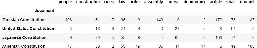
Since our texts are all constitutions, we could have a look at some intriguing terms.
But, what else should we be checking? Which words might be the most interesting? The idxmax pandas method would return the label of the column with the maximum value, for each row. That is, we’ll get the most frequent word for each document.
counts.idxmax(axis=1)
document
Tunisian Constitution         article
United States Constitution      shall
Japanese Constitution           shall
Athenian Constitution         council
dtype: object
Now, we look at this subset of words accross all documents.
counts[['people','constitution', 'rules', 'law', 'order', 'assembly', 'house', 'democracy','article','shall','council']]
Term Frequency
We’re going to take into account how often a term shows up by using the TfidfVectorizer in the same way as CountVectorizer. TfidfVectorizer converts a collection of documents to a matrix of TF-IDF features. It is equivalent to CountVectorizer followed by TfidfTransformer.
tfidf_vectorizer = TfidfVectorizer(stop_words='english', use_idf=False)

x = tfidf_vectorizer.fit_transform(df.content)
tfidfcounts = pd.DataFrame(x.toarray(),index = df.document, columns = tfidf_vectorizer.get_feature_names())
Let’s check the same words as we did before!
tfidfcounts[['people','constitution', 'rules', 'law', 'order', 'assembly', 'house', 'democracy','article','shall','council']]
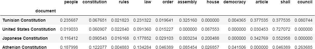
Notice how our numbers have shifted a bit. These are supposedly better relative indicators for the use of words, and their importance in our documents.
Inverse document frequency
By looking at the previous DataFrame, it seems like the word (shall) shows up a lot. So, even though it’s not a stopword, it should be weighted a bit less.
This is inverse term frequency. The more frequent a term shows up across documents, the less important it can be in our matrix.
#use_idf bool, default=True (to highlight by comparison) Enable inverse-document-frequency reweighting
idf_vectorizer = TfidfVectorizer(stop_words='english', use_idf=True)

y = idf_vectorizer.fit_transform(df.content)
idfcounts = pd.DataFrame(y.toarray(), index = df.document, columns = idf_vectorizer.get_feature_names())
Again with the same subset of words accross all documents.
idfcounts[['people','constitution', 'rules', 'law', 'order', 'assembly', 'house', 'democracy','article','shall','council']]

Notice how (council) increased in value because it’s an infrequent term, and (people) decreased in value because it’s quite frequent.
It is beneficial to understand how TF-IDF functions in order to obtain a deeper understanding of how machine learning algorithms work. TF-IDF allows us to associate each word in a document with a numerical value or vector, that reflects its relevance in that document.
In text analysis with machine learning, TF-IDF algorithms help extract keywords, and by determining similar documents, we are able to automatically sort them into clusters.
Besides, given a query, variations of the TF-IDF weighting are also used by search engines in scoring and ranking a document’s relevance.
Leave a comment