K-Means clustering and similarity visualization of constitutions

• Introduction
• Text processing and exploratory analysis
• K-Means clustering
• Visualizing text corpus similarity

---

Introduction

Constitutions hold the fundamental principles and rules that constitute the legal basis of a country. They determine the system of goverment, and the relationships between branches and institutions.

When written, these documents can be quite unique and distinct in many aspects, such as length and legal terminology. However, they can also share some other features, since they tend to have similar purposes.

A textual analysis of such data can be useful. We are going to apply some techniques to compare and cluster various constitutions. This work tries to see if constitutional text corpuses are indicative of the set and outlined systems of government.

To do so, we are going to use TF-IDF term weighting and K-Means clustering from scikit-learn. If you need a text analysis refresher, please check here.

---

# importing the libraries
import os
import pandas as pd
from sklearn.feature_extraction.text import TfidfVectorizer
from sklearn.cluster import KMeans

%matplotlib inline

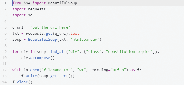
There are 35 constitutions in our dataset. Most of the documents were queried from constitute project on April 2021, using a simple crawler that implements the Beautiful Soup library.

If you intend on getting your data from the source above, and as a general good scraping etiquette, please be nice and avoid overburdening their servers with requests.

After importing the necessary libraries, we read our documents to a DataFrame.

# Construct an empty DataFrame with two columns
df = pd.DataFrame(columns=('document', 'content'))
# Go through the files in working directory
# If it's a text file, open it and append the content to the DataFrame
for filename in os.listdir(os.getcwd()):
    if filename.endswith('.txt'):
        df = df.append({"document": filename[:len(filename)-4],
                        "content": open(filename, encoding='latin_1').read().replace("\n"," ")},
                       ignore_index=True)

We should check the names of the documents. Since pandas DataFrame columns are Series, we can pull them out and call .tolist() to turn them into a Python list.

print(df['document'].tolist())

['algeria_constitution', 'australia_constitution', 'austria_constitution', 'belgium_constitution', 'brazil_constitution', 'burkinafaso_constitution', 'china_constitution', 'costarica_constitution', 'ecuador_constitution', 'france_constitution', 'germany_constitution', 'india_constitution', 'japan_constitution', 'korea_constitution', 'malaysia_constitution', 'mexico_constitution', 'morocco_constitution', 'netherlands_constitution', 'nigeria_constitution', 'norway_constitution', 'pakistan_constitution', 'peru_constitution', 'portugal_constitution', 'rwanda_constitution', 'senegal_constitution', 'singapore_constitution', 'southafrica_constitution', 'spain_constitution', 'sweden_constitution', 'switzerland_constitution', 'tunisia_constitution', 'turkey_constitution', 'us_constitution', 'vietnam_constitution', 'zambia_constitution']

As we can see, the constitutions pertain to different countries from around the world, with different systems of government. Some nations from the list are monarchies, others are republics. Some have a unitary government, while others are federal. And the differences extend to the legislature as well.
It is, in fact, a diverse collection. But, we should keep in mind that most of these constitutions are translated from their respective native languages. The original meaning in each document may not be conveyed with the same degree of accuracy.

---

Text processing and exploratory analysis

Next, we begin the analysis.
First, we choose a list of stopwords from the Natural Language Tolkit project (nltk). These are high-frequency terms (like who and the), that we may want to filter out of documents before processing.

from nltk.corpus import stopwords
sw = stopwords.words('english')
sw.append('shall') # Add "shall" to stopwrods
print ("There are", len(sw), "words in this stopwords list. The first 10 are:", sw[:10])

There are 180 words in this stopwords list. The first 10 are: ['i', 'me', 'my', 'myself', 'we', 'our', 'ours', 'ourselves', 'you', "you're"]

Then, we are going to tokenize our texts. NLTK provides several types of tokenizers for that purpose. We will use a custom regular expression tokenizer, that detects words containing alphanumeric characters only.

from nltk import regexp_tokenize
patn = '\w+'
df['content'] = df['content'].apply(lambda w: " ".join(regexp_tokenize(w, patn)))

To have better insights from our text corpus, let us create 4 new columns:

• df['number_words'] for the number of words in each document
• df['unique_words'] for the number of unique words in each document
• df['number_words_without_sw'] for the number of words that are not in the stopwords list
• df['percentage'] for the percentage of stop words in each text corpus

df['unique_words'] = df['content'].apply(lambda x: len(set(x.split())))
df['number_words'] = df['content'].apply(lambda x: len(x.split()))
df['number_words_without_sw'] = df['content'].apply(lambda y: len([word for word in y.split() if word not in sw]))
df['percentage'] = 100 - (df['number_words_without_sw'] * 100 / df['number_words'])

Let us use .head() to preview the first 6 rows of our DataFrame.

df.head(6)

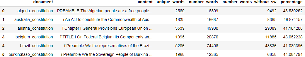
All of the percentage values are less than 50. In fact, we can surmise that a well written piece of legal document, should not have a lot of stopwords. However, that may not always be the case. Feel free to share your opinions regarding this, in the comments section below, or by email.

We can push the exploration further, and check which constitutions have the most and the least unique words. Such a measure can be an indicator of the richness of the used lexicon, and its complexity as well.

max_unique_words = df['unique_words'].max()
doc_max_unique_words = df['document'][df.index[df['unique_words'].idxmax()]]
min_unique_words = df['unique_words'].min()
doc_min_unique_words = df['document'][df.index[df['unique_words'].idxmin()]]

print ("The {} has the most unique words with {} words. And the {} has the fewest with only {}"
       .format(doc_max_unique_words, max_unique_words, doc_min_unique_words, min_unique_words))

The brazil_constitution has the most unique words with 5286 words. And the us_constitution has the fewest with only 1005

---

After the previous exploratory phase, we move to term weighting and tf-idf.

Like we did in the previous article linked above, we are going to use TfidfVectorizer from sklearn to convert the collection of documents to a matrix of TF-IDF features. That would allow us to take into account how often a term shows up.
Again, tf-idf is a statistical measure that evaluates how relevant a word is to a document in a collection of documents. You can refer to the official sklearn documentation for the complex mathematical explanation.

tfidf_vectorizer = TfidfVectorizer(stop_words=sw, use_idf=True)

x = tfidf_vectorizer.fit_transform(df.content)
tfidfcounts = pd.DataFrame(x.toarray(),index = df.document, columns = tfidf_vectorizer.get_feature_names())

---

K-Means clustering

Let us go over a brief explanation of clustering in general before delving into K-Means clustering that we will be using.

Clustering is the process of grouping a collection of objects, such that those in the same partition (or cluster) are more similar (in some sense) to each other, than to those in other groups (clusters).
There are a lot of clustering algorithms that can be utilized, and their use is modulated by specific conditions in the use cases.

As for the K-Means algorithm, it clusters data by trying to separate samples in n groups of equal variance. It minimizes the squared distance between the cluster mean (centroid) and the points in the cluster. This algorithm requires the number of clusters to be specified.

Below, we set the desired number of clusters. That choice is not an easy task. There are a few ways to determine the optimal number of clusters, but for the sake of this demonstration, we will not be going through them.

# Specify number of clusters
number_of_clusters = 3
km = KMeans(n_clusters = number_of_clusters)
# Compute k-means clustering
km.fit(x)

KMeans(n_clusters=3)

After computing the k-means clustering, and getting a fitted estimator, we ought to see the top words in each cluster.
In the code below, cluster_centers_ gets the coordinates of each centroid. Then, .argsort()[:, ::-1] converts each centroid into a descending sorted list of columns by their relevance. That gives the words most relevant, since in our vector representation, words are the features in the form of columns.
We use .get_feature_names() to get a list of feature names mapped from feature integer indices.
Finally, the for loop wraps up the work, and prints out the top words in each cluster.

order_centroids = km.cluster_centers_.argsort()[:, ::-1]
terms = tfidf_vectorizer.get_feature_names()

for i in range(number_of_clusters):
    top_words = [terms[ind] for ind in order_centroids[i, :5]]
    print("Cluster {}: {}".format(i, ' '.join(top_words)))

Cluster 0: state may federal law section
Cluster 1: article law national state president
Cluster 2: federal art law confederation para

The top terms for each cluster are somewhat intriguing. In fact, certain words do pertain to specific systems of government.
Let us check the full results, and see how the entire dataset was partitioned.

results = pd.DataFrame()
results['document'] = df.document
results['category'] = km.labels_
results

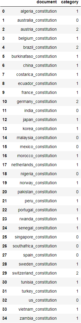
By observing the results and seeing the top words for each cluster, we can see that a lot of Federal countries were assigned to cluster 2. However, a few were put in other clusters. By the same, some non-Federal countries were grouped in cluster 2.
The same goes for clusters 0 and 1, where similar systems of government are not always put together.

This suggests that word relevance on its own, just gives a broader perception of how well the text corpus reflects the system of government.
The analysis can be improved by using other algorithms and techniques. However, K-Means clustering being fairly simple and easy to implement, can be a good starting point for further and deeper inspection.

---

Visualizing text corpus similarity

We can visualize the similarities based on the TF-IDF features.
To do so, we start by constructing the vectorizer as usual. We specify max_features to build a vocabulary that considers only the top max_features ordered by term frequency across the dataset.

vectorizer = TfidfVectorizer(use_idf=True, max_features=10, stop_words=sw)
X = vectorizer.fit_transform(df.content)
print (vectorizer.get_feature_names())

['article', 'constitution', 'court', 'federal', 'law', 'may', 'national', 'president', 'public', 'state']

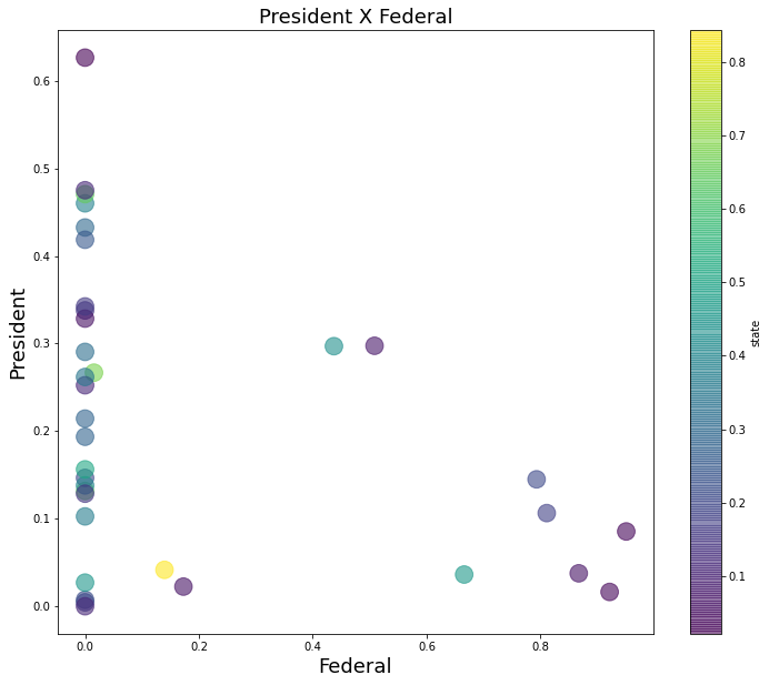
We can use a combination of DataFrame.plot and matplotlib to draw a scatter plot representing the distribution of two terms on x and y axes, and a colormap to showcase the rlevance of a third term.
We can clearly see than only 10 data points had some value regarding the term federal, while the rest had a value of 0 or close.

df2 = pd.DataFrame(X.toarray(), columns=vectorizer.get_feature_names())
import matplotlib.pyplot as plt
fig = plt.figure()
axi = plt.gca()

ax = df2.plot(kind='scatter', x= 'federal', y= 'president', s= 250, alpha= 0.6,
              c='state', colormap='viridis',
              figsize= (12,10), ax= axi)

axi.set_title('President X Federal', fontsize=18)
axi.set_xlabel("Federal", fontsize=18)
axi.set_ylabel("President", fontsize=18)

Text(0, 0.5, 'President')